Reports

Contents

Title: Camera comparison at Mayberry
Date:2022-02-17
Data File: MBautocam_20220217.csv
MBpicam_20220217.csv
MBpicamFWB_20220217.csv
MBstardot_20220217.csv
Refers to:RPI0W-003,0030F4D214A4
Starting in May 2021, we set up several cameras on the Mayberry tower to compare their GCC results. Besides the Autocam (Canon) camera that has been running forever there, we added a Raspberry Pi camera (Picam) in May and a Stardot camera in June. The Stardot camera is the official camera of the Phenocam network and it is set with a fixed white balance. The Autocam and the Picam have a dynamic white balance that the camera adjusts according to the light conditions.
 
Since the initial Picam data was kind of noisy, Joe set up the Picam to save 2 photos from each time point, 1 photo with a dynamic white balance and 1 photo with a fixed white balance (FWB). Starting in September, there are 2  "Picam" data series in the figures. The hope is that the FWB would reduce the noise in the Picam data.
  • Picam = picam photo with dynamic white balance
  • Picam FWB = picam photo with fixed white balance
 
For this analysis, I defined midday as 11:15-13:15, inclusive. The comparison ended on 2022-02-17 when I removed the Canon autocam from the tower to bring back to the lab for testing. The Canon photos were consistently underexposed/dark during some daytime hours.
 
Summary:
  • The Stardot camera and the Picam with FWB have similar fits with the Autocam data, so either could be used to fill the Autocam data.
  • For filling in missing Autocam data in Oct/Nov 2021, use this relationship with the Stardot camera. AutocamGCC=0.964*(StardotGCC)+0.013
  • If using a Picam camera at a site, using a fixed white balance substantially reduces noise (R2 increased from 76% to 96% when using fixed white balance)
  • If the absolute GCC is important when using the Picam with fixed white balance, the Red, Green, Blue gains should be adjusted so that the GCC values match the reference GCC.


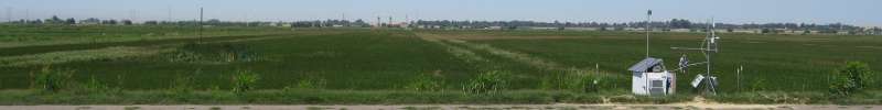
All 3 cameras (and the diffuse PAR sensors) on the same post on the Mayberry tower. Cameras are facing west.


16458395415645.png
Fig 1. Time series of midday GCC calculated from various cameras. Overall the 3 cameras have GCC that actually match pretty well. Picam FWB is offset from the GCC, which is ok because we could adjust the gains for R, G, B to have it match the GCC of the other cameras. In general we are interested in the relative GCC at our sites, not necessarily the absolute GCC.
 
All data
 
First, I was interested in how well we can use other cameras to fill in the gaps in the Autocam data so I plotted the linear regression lines. There is a big chunk of Autocam data missing in Oct/Nov 2021, so it would be nice to fill it in with something before running the ANN (if GCC is one of the predictor variables).
 
16458398687654.png
Fig 2. Linear regression between Picam GCC and Autocam GCC. Some scatter around the line but there's a definite relationship with R2=92%.
 
16458398814085.png
Fig 3. Linear regression between Picam FWB GCC and Autocam GCC. Two groupings of data from either super green vegetation or senesced vegetation. The Picam was killed by the power issues in the fall so there was no Picam data from most of November 2021.
 
16458398925326.png
Fig 4. Linear regression between Stardot GCC and Autocam GCC. This has the best fit with R2=98%. For filling in missing Autocam data in Oct/Nov, I would use this relationship with the Stardot camera since Stardot data is available during that time chunk.
 
AutocamGCC=0.964*(StardotGCC)+0.013
 
 
In general, the linear fits are all pretty good, with slopes within 20% of 1, offsets ~0, and R2>90%. However, Figure 2 shows the Picam data is a lot messier than the Picam FWB or the Stardot data.
 
Data subset - only when all 3 cameras were running
 
Since the cameras were up for different lengths of time, I want to control the "n" in the R2 calculation when I compare all three. I restricted my analysis to the days when all 3 cameras had data. This turned out to be 94 days (not continuous) between 2021-09-15 and 2022-02-27.
 
16458401010124.png
Fig 5. Linear regression between Picam and Autocam GCC for a subset of dates when all 3 camera types were running. R2 is markedly lower with R2 at only 76%. Data from senescent vegetation is more heavily weighted here than when looking at the whole time series. When the vegetation has already senesced, there's not much change in GCC, and the Picam signal to noise ratio gets worse (more noise).
 
16458401122360.png
Fig 6. Linear regression between Picam FWB and Autocam GCC. The R2 (96%) here is much better than the R2 (76%) when comparing Picam (dynamic WB) and Autocam GCC in Fig 5.
 
16458401227719.png
Fig 7. Linear regression between Stardot GCC and Autocam GCC. The fit is still very good (R2=98%) and is comparable to the fit between Picam FWB and Autocam GCC (R2=96%). Given the cost differences between the Stardot camera (0+) and the Picam (~0), the Picam FWB seems like a decent substitute for the Stardot camera. The downside to the Pi Zero W is that it can be hard to find.
 
MATLAB Code

%% CamIntercompare.m
% This script loads .csv files of camera data and uses the function
% middayGCC.m to calculate midday GCC based on a start and end time input
% into the function.

% The objective of this study was to compare GCC values and stability
% across different types of cameras. Can another camera used to fill gaps
% in Autocam data, or replace the Autocam all together?

close all
clear all

f=load('MBautocam.csv');
yr=f(:,1);
doy=f(:,2);
hhmm=f(:,3);
red=f(:,5);
grn=f(:,6);
blu=f(:,7);
[t_a,gcc_mid_a]=middayGCC(yr,doy,hhmm,red,grn,blu,1115,1315);

f=load('MBpicam.csv');
yr=f(:,1);
doy=f(:,2);
hhmm=f(:,3);
red=f(:,5);
grn=f(:,6);
blu=f(:,7);
[t_p,gcc_mid_p]=middayGCC(yr,doy,hhmm,red,grn,blu,1115,1315);

f=load('MBpicamFWB.csv');
yr=f(:,1);
doy=f(:,2);
hhmm=f(:,3);
red=f(:,5);
grn=f(:,6);
blu=f(:,7);
[t_pf,gcc_mid_pf]=middayGCC(yr,doy,hhmm,red,grn,blu,1115,1315);

f=load('MBstardot.csv');
yr=f(:,1);
doy=f(:,2);
hhmm=f(:,3);
red=f(:,5);
grn=f(:,6);
blu=f(:,7);
[t_s,gcc_mid_s]=middayGCC(yr,doy,hhmm,red,grn,blu,1115,1315);

figure();
plot(t_a, gcc_mid_a, 'g.', 'markersize',10);
hold on;
plot(t_p, gcc_mid_p, 'r.', 'markersize',10);
plot(t_pf, gcc_mid_pf, 'm.', 'markersize',10);
plot(t_s, gcc_mid_s, 'c.', 'markersize',10);
ylabel('GCC');
legend('Autocam', 'Picam', 'Picam Fixed WB', 'Stardot', 'Location', 'Northwest');
title('Mayberry GCC w/ various cameras')

%% Intersection of all 4 arrays

[i,ia,is]=intersect(t_a,t_s);
[j,jx,jy]=intersect(t_p,t_pf);
[k,kx,ky]=intersect(i,j);

[d,dx,dy]=intersect(t_a, k);
t_a_sub=t_a(dx);
gcc_mid_a_sub=gcc_mid_a(dx);

[d,dx,dy]=intersect(t_s, k);
t_s_sub=t_s(dx);
gcc_mid_s_sub=gcc_mid_s(dx);

[d,dx,dy]=intersect(t_p, k);
t_p_sub=t_p(dx);
gcc_mid_p_sub=gcc_mid_p(dx);

[d,dx,dy]=intersect(t_pf, k);
t_pf_sub=t_pf(dx);
gcc_mid_pf_sub=gcc_mid_pf(dx);


%% Regression: Picam vs. Autocam
x=t_p;
y=t_a;
[i,ix,iy]=intersect(x,y);
% i=x(ix);
% i=y(iy);
x=gcc_mid_p(ix);
y=gcc_mid_a(iy);

mdl=fitlm(x,y);

figure();
plot(x,y, 'rx'); hold on; plot([min(x) max(x)],[min(x)*mdl.Coefficients.Estimate(2)+mdl.Coefficients.Estimate(1) max(x)*mdl.Coefficients.Estimate(2)+mdl.Coefficients.Estimate(1)]);
legend('Data', sprintf('Model y=%0.3fx + %0.3f, R^2=%0.1f, n=%d',mdl.Coefficients.Estimate(2),mdl.Coefficients.Estimate(1),mdl.Rsquared.Ordinary*100, mdl.NumObservations), 'Location', 'Northwest');
ylabel('Autocam GCC')
xlabel('Picam GCC')
title('Autocam vs. Picam')


x=gcc_mid_p_sub;
y=gcc_mid_a_sub;
mdl=fitlm(x,y);

figure();
plot(x,y, 'rx'); hold on; plot([min(x) max(x)],[min(x)*mdl.Coefficients.Estimate(2)+mdl.Coefficients.Estimate(1) max(x)*mdl.Coefficients.Estimate(2)+mdl.Coefficients.Estimate(1)]);
legend('Data', sprintf('Model y=%0.3fx + %0.3f, R^2=%0.1f, n=%d',mdl.Coefficients.Estimate(2),mdl.Coefficients.Estimate(1),mdl.Rsquared.Ordinary*100, mdl.NumObservations), 'Location', 'Northwest');
ylabel('Autocam GCC')
xlabel('Picam GCC')
title('Autocam vs. Picam (only dates where all 3 cameras running)')

%% Regression: Picam with FWB vs. Autocam
x=t_pf;
y=t_a;
[i,ix,iy]=intersect(x,y);
% i=x(ix);
% i=y(iy);
x=gcc_mid_pf(ix);
y=gcc_mid_a(iy);

mdl=fitlm(x,y);

figure();
plot(x,y, 'mx'); hold on; plot([min(x) max(x)],[min(x)*mdl.Coefficients.Estimate(2)+mdl.Coefficients.Estimate(1) max(x)*mdl.Coefficients.Estimate(2)+mdl.Coefficients.Estimate(1)]);
legend('Data', sprintf('Model y=%0.3fx + %0.3f, R^2=%0.1f, n=%d',mdl.Coefficients.Estimate(2),mdl.Coefficients.Estimate(1),mdl.Rsquared.Ordinary*100, mdl.NumObservations), 'Location', 'Northwest');
ylabel('Autocam GCC')
xlabel('Picam FWB GCC')
title('Autocam vs. Picam FWB')


x=gcc_mid_pf_sub;
y=gcc_mid_a_sub;
mdl=fitlm(x,y);

figure();
plot(x,y, 'mx'); hold on; plot([min(x) max(x)],[min(x)*mdl.Coefficients.Estimate(2)+mdl.Coefficients.Estimate(1) max(x)*mdl.Coefficients.Estimate(2)+mdl.Coefficients.Estimate(1)]);
legend('Data', sprintf('Model y=%0.3fx + %0.3f, R^2=%0.1f, n=%d',mdl.Coefficients.Estimate(2),mdl.Coefficients.Estimate(1),mdl.Rsquared.Ordinary*100, mdl.NumObservations), 'Location', 'Northwest');
ylabel('Autocam GCC')
xlabel('Picam FWB GCC')
title('Autocam vs. Picam FWB (only dates where all 3 cameras running)')

%% Regression: Stardot vs. Autocam
x=t_s;
y=t_a;
[i,ix,iy]=intersect(x,y);
% i=x(ix);
% i=y(iy);
x=gcc_mid_s(ix);
y=gcc_mid_a(iy);

mdl=fitlm(x,y);

figure();
plot(x,y, 'cx'); hold on; plot([min(x) max(x)],[min(x)*mdl.Coefficients.Estimate(2)+mdl.Coefficients.Estimate(1) max(x)*mdl.Coefficients.Estimate(2)+mdl.Coefficients.Estimate(1)]);
legend('Data', sprintf('Model y=%0.3fx + %0.3f, R^2=%0.1f, n=%d',mdl.Coefficients.Estimate(2),mdl.Coefficients.Estimate(1),mdl.Rsquared.Ordinary*100, mdl.NumObservations), 'Location', 'Northwest');
ylabel('Autocam GCC')
xlabel('Stardot GCC')
title('Autocam vs. Stardot')


x=gcc_mid_s_sub;
y=gcc_mid_a_sub;
mdl=fitlm(x,y);

figure();
plot(x,y, 'cx'); hold on; plot([min(x) max(x)],[min(x)*mdl.Coefficients.Estimate(2)+mdl.Coefficients.Estimate(1) max(x)*mdl.Coefficients.Estimate(2)+mdl.Coefficients.Estimate(1)]);
legend('Data', sprintf('Model y=%0.3fx + %0.3f, R^2=%0.1f, n=%d',mdl.Coefficients.Estimate(2),mdl.Coefficients.Estimate(1),mdl.Rsquared.Ordinary*100, mdl.NumObservations), 'Location', 'Northwest');
ylabel('Autocam GCC')
xlabel('Stardot GCC')
title('Autocam vs. Stardot (only dates where all 3 cameras running)')


function [t,gcc_mid_avg] = middayGCC(yr,doy,hhmm,red,grn,blu,hhmm1,hhmm2)
%middayGCC Calculate GCC given RGB and start/end time
% OUTPUTS
% t = timestamp of GCC in datetime format(time is hardcoded to 12:00 for now)
% gcc_mid_avg = midday GCC average with midday defined as tod1<=t=>tod2
% INPUTS
% yr = year of data (to calculate datetime)
% doy = day of year of data
% hhmm = hour and minute in hhmm format
% red = red
% grn = green
% blu = blue
% hhmm1 = start time in hhmm format (minimum time included, INCLUSIVE)
% hhmm2 = end time in hhmm format (maximum time included, INCLUSIVE)

gcc=grn./(red+grn+blu);

i=find((hhmm>=hhmm1) & (hhmm<=hhmm2));
gcc_mid=gcc(i);
doy_mid=doy(i);
yr_mid=yr(i);
doy_mid=datetime(yr_mid,1,doy_mid);

[doy_mid_unique,ia,ic] = unique(doy_mid);
%doy_mid_unique=doy_mid(ia)
%doy_mid=doy_mid_unique(ic)
gcc_mid_avg=accumarray(ic,gcc_mid,[],@mean);
t=datetime((datenum(doy_mid_unique) + datenum(0,0,0,12,0,0)),'convertfrom', 'datenum');
end