Reports

Picam sn RPI0W-005 ("old picam") and sn RPI0W-006 ("new picam") were compared at East End over 4 months.

We had noticed that the photos from sn RPI0W-005 were looking washed out. We observed that the East End canopy was getting taller through the years and reaching the same height as the "old picam" sn RPI0W-005, which was attached to the upper level of the scaffolding, so we wanted to install another camera that was higher up on the tower.

On 2024-05-01, we installed the "new picam" sn RPI0W-006 on the 7500 mount, maybe 50cm higher than the "old picam"

EE_cam data in database since 2024-05-01 is from the "new picam" sn RPI0W-006.

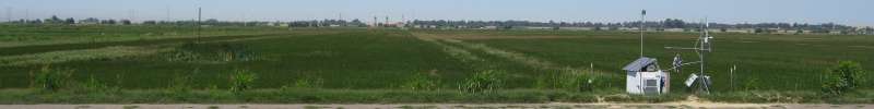
Figure 1. 2018 and 2023 photos of the East End tower show the dramatic increase in canopy height.

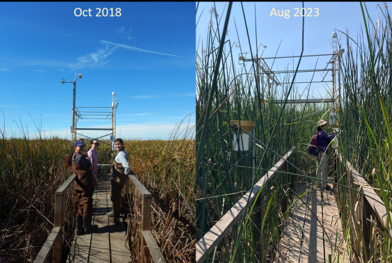
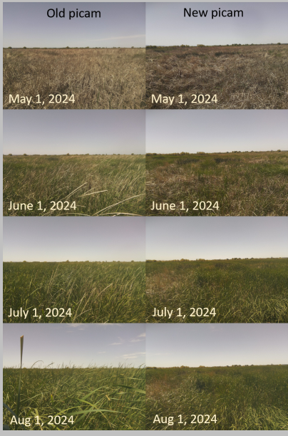
Figure 2. Comparison of photos from the first of each month, May through August. "Old" picam photos in the left column and "new" picam photos in the right column. Each photo is from 12:45 PST. Near the end of the growing season, the canopy is at the same height as the "old" picam.

When the canopy is closer to the camera, we see more of the flat side of the leaf (the face of the leaf)as opposed to the edges of the leaf. I think this makes the GCC value lower overall because the color of the leaf face is lighter then the leaf edge. We also see fewer leaves in general when the canopy is close to the camera.

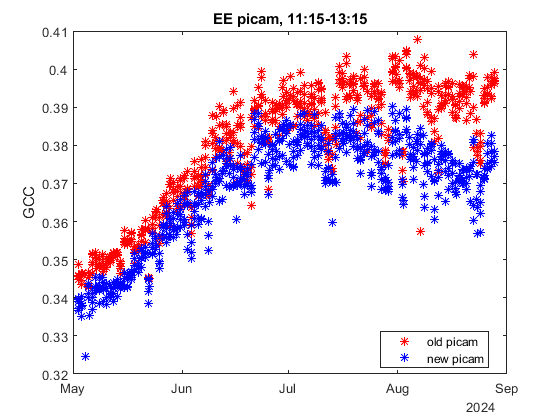
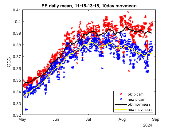
Figure 3. Time series of GCC values from each picam, with each symbol representing one photo. There are 5 photos from each day: 11:15, 11:45, 12:15, 12:45, and 13:15 PST. At the start of the comparison period, the GCC from both cameras is very similar, but they get more different as time passes. The "old" picam has a lower GCC than the "new" picam by mid-August.

Figure 4. Time series of GCC from both picams. The 5 values from each day were averaged, and the daily average was used to calculate the 10-day running mean (bold line). Here we see the running means started deviating from each other in mid July.

The weird thing is that even though the canopy is clearly greening up from May through August (as seen in the photos), the overall GCC trend is flat/downward. Maybe this is just from all of the noise in the picam photos with auto white balance? I do have the fixed white balance picam photos, maybe I should compare those and see if it's any better.

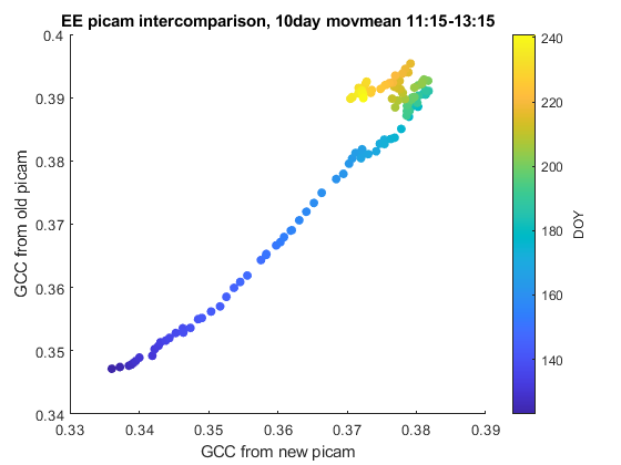
Figure 5. Scatter plot of GCC from each camera. The symbols are colored based on the DOY (see colorbar on the right axis). If you follow the points from earlier dates (dark purple) to later dates (bright yellow), the scatter plot makes a zig zag pattern. Slope of the scatter stays similar, but the offset changes about through time. Joe thinks this is because as the canopy grew taller, the view angle of the cameras changed.

Conclusion: Camera's view angle does impact our calculated GCC.

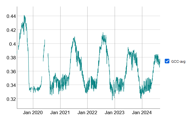
Figure 5. Timeseries of of GCC data from EE_cam starting June 2019. The camera changed twice during this period, Jul 2020 (Stardot to "old picam") and May 2024 ("old picam" to "new picam"). Interesting that the summer peak in 2023-2024 are lower than summer peaks 2021-2022, although it was the one picam 2021-2023 and a different picam in 2024. Maybe the litter building up over the years is decreasing the max summer GCC.

2020-07-21: "Old picam" sn RPI0W-005 installed to replace stolen Stardot camera

2024-05-01: "New picam" sn RPI0W-006 installed

---------------------------------Code ---------------------------------

clear variables;
close all;

% Load inputs
old=readtable('oldEEpicam_2024.csv');
t_old=old.t_old;
dt_old=datetime(t_old,'convertfrom','datenum');
old=old.old;
new=readtable('newEEpicam_2024.csv');
t_new=new.t_new;
dt_new=datetime(t_new,'convertfrom','datenum');
new=new.new;

[old_avg,old_day]=dailyMean(old,t_old);
[new_avg,new_day]=dailyMean(new,t_new);

[old_mdn,~]=dailyMedian(old,t_old);
[new_mdn,~]=dailyMedian(new,t_new);

dt_old_day=datetime(old_day,'convertfrom','datenum');
dt_new_day=datetime(new_day,'convertfrom','datenum');

figure();
plot(dt_old,old,'r*');
hold on;
plot(dt_new,new,'b*');
title('EE picam, 11:15-13:15')
ylabel('GCC')
legend('old picam','new picam')

figure();
plot(dt_old,old,'r*');
hold on;
plot(dt_new,new,'b*');
plot(dt_old_day,old_avg, 'r-');
plot(dt_new_day,new_avg,'b-');
title('EE daily mean, 11:15-13:15')
ylabel('GCC')
legend('old picam', 'new picam', 'old median', 'new median');

new_avg5=movmean(new_avg,5);
old_avg5=movmean(old_avg,5);

figure();
plot(dt_old,old,'r*');
hold on;
plot(dt_new,new,'b*');
plot(dt_old_day,old_avg5,'r-','linewidth',2);
plot(dt_new_day,new_avg5,'b-','linewidth',2);
title('EE daily mean, 11:15-13:15, 5day movmean')
ylabel('GCC')
legend('old picam','new picam','old movmean','new movmean');

%[C,ia,ib] = intersect(a,b)
% C = A(ia) and C = B(ib)

[t_int,i_new,i_old]=intersect(new_day,old_day);
dt=datetime(t_int,'convertfrom','datenum');
dy=day(dt,'dayofyear')';

figure();
scatter(new_avg5(i_new),old_avg5(i_old),[],dy,'filled');
c=colorbar;c.Label.String='DOY';
xlabel('GCC from new picam')
ylabel('GCC from old picam')
title('EE picam intercomparison, 5day movmean 11:15-13:15')