Reports
Contents
| Title: | Zcam gap fraction at Bouldin Corn | ||||||||||||||||
| Date: | 2020-08-18 | ||||||||||||||||
| Data File: | BC_zcam_2019.csv BC_zcam_2020.csv BC_zcam_20192020.csv |
||||||||||||||||
| Refers to: | BC, RPI0W-001,RPI0W-002, RPI0W-004 | ||||||||||||||||
|
In summers 2019 and 2020, we tested 2 different methods of continuously measuring canopy gap fraction at Bouldin Corn. We tested 2 types of upward looking sensors: lost-cost Raspberry Pi cameras and Kipp & Zonen PAR sensors. Could we use these continuous measurements as a proxy for labor-intensive manual measurements? Can we use continuous gap fraction measurements to estimate the light extinction coefficient? Our usual manual measurements -LAI using a LI-3100 with destructively sampled leaves -PAI using a handheld LAI-2200C -Aboveground biomass with destructively sampled plants -Vegetation height using a measuring tape Our continuous measurements -Raspberry Pi cameras (zcams) that are on the ground, looking upwards through the canopy. In 2019 we had 2 regular-lens cameras. In 2020 we had 1 regular-lens camera and 2 wide-lens cameras. Joe customized the MATLAB script he uses for the Tonzi zcams to calculate gap fraction from the midday Raspberry Pi photos. In short, because sky pixels are bright and leaf pixels are dark, the script calculates a bimodal histogram of pixel brightness. It uses the minimum point between the 2 modes to classify each pixel as dark or bright and then calculate gap fraction as the ratio of bright to dark pixels. -PAR sensors (zPAR) that are on the ground, looking upwards through the canopy. We had 2 sensors in 2020; none in 2019. To make this data useful for analysis, Joe first took the daily sum of total incoming PAR and the 2 under canopy PAR sensors. He then divided the under canopy sum by the incoming sum to account for cloudiness and different holes in the canopy as the sun moved across the sky.
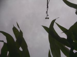
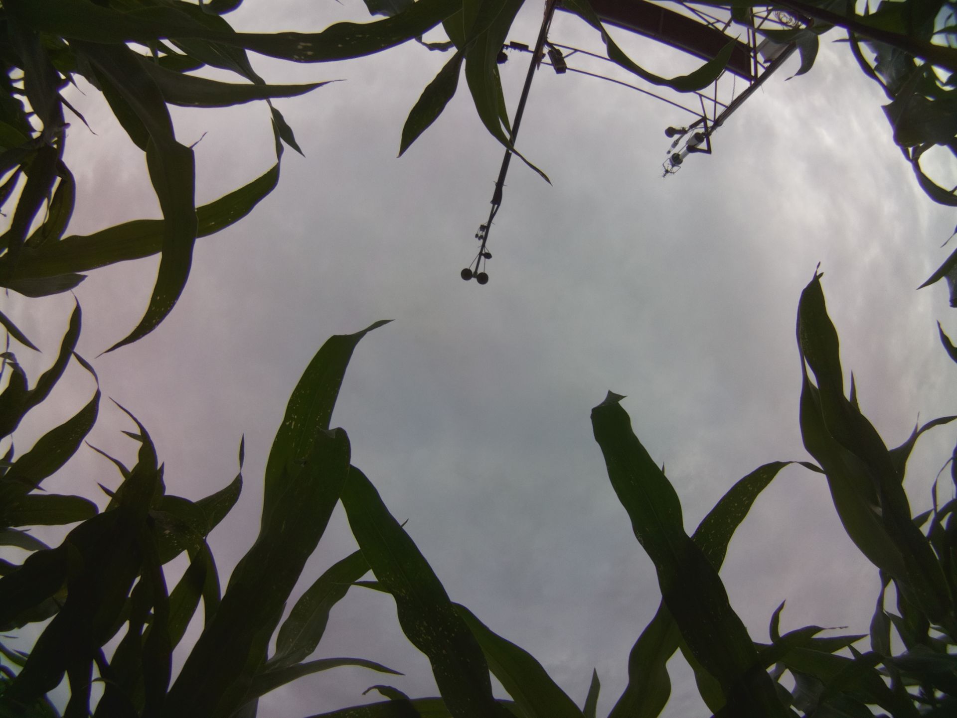
(L) Photo from Raspberry Pi zcam with regular lens. The leaves (and radiometer boom) are dark while the sky is bright. (R) Photo from Raspberry Pi zcam with wide lens taken at same day and time. The two cameras are a meter apart.
Beer's law and the light extinction coefficient Beer's law tells us:
I(L) = I0 * exp (-k * L)
I(L) = Radiation at bottom of canopy as a function of LAI
I0 = Radiation at top of canopy
k = Extinction coefficient
L = LAI
If we take the natural log of both sides of the equation, we get:
ln (I(L)/I0) = -k * L
From our zcams, we have estimated gap fraction, or the probability that radiation at the top of the canopy will reach the bottom of the canopy without hitting any part of the canopy. I(L)/I0 = gap fraction
ln (gap fraction) = -k * L
So we can use the slope of these figures to look at the light extinction coefficient (k).
2019 In 2019 we had 2 Raspberry Pi cameras with regular lenses. The corn was planted on 2020-05-25, 25 days before the start of the graph. The gap fraction mostly saturated in the first month of growth, about 6 weeks after planting. The gap fraction decreased from 1 to 0.1 over 3 weeks, corresponding to veg height increasing from 40 to 165 cm. The messiness at the end of June is caused by leaves moving in and out of the camera lens, especially leaves right above the lens. There was a weed with large, flat leaves growing right above ZCam2. The corn plant seemed to reach full leaf-out about 45 days after planting (2020-07-09), and maximum LAI about 55-65 days (around 2020-08-08) after planting. They harvested most of the corn field on 2020-09-14 (~90 days after planting).
Figure 1. Daily average gap fraction from 2 different zcams.
Figure 2. Natural log of daily average gap fraction. The slope (light extinction coefficient) of this regression with PAI is -0.35 and the R2 was 0.79. We did not have enough points to calculate a regression between LAI and gap fraction.
2020 In 2020 we had 2 Raspberry Pi cameras with wide angle (fish eye) lenses and 1 camera with a regular lens. The corn management timing was quite different in 2020 compared to 2019. In 2020, the corn was planted on 2020-04-30, almost 2 months earlier than the previous year. The corn sprouted 9 days after planting and the gap fraction saturates about 2 months later around 2020-06-28. They farmers on 2020-10-12, almost 6 months after planting.
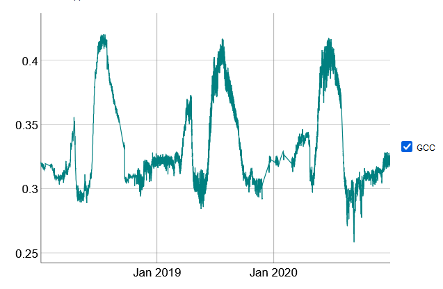
Multi-year plot of GCC at the site shows how the corn growing season was much earlier in 2020 compared to the previous two years.
Figure 3. Daily average gap fraction from 3 zcams. The wide and regular lens cameras agree well. Although the wide lens has a distorted view compared to the regular lens, we don't need to correct for the distortion because gap fraction is the ratio of area of leaves to the area of sky. In a given area, the leaf area and sky area are distorted in the same way. There's quite a bit of variation between the two LAI methods. Most days there was ~0.75 difference in LAI between the two methods, but it's inconsistent which method gives the higher LAI. We had 4 different people make these measurements on different days. This probably shows how sensitive these measurements are to protocol, even though we tried to standardize our methodology. We probably need to sample more than 5 plants for LAI in the future.
Figure 4. The slope (light extinction coefficient) of the 2 manual methods are similar, -0.37 and -0.39. R2 is 0.82 and 0.88. These are slightly steeper than the slope from last year's PAI regression, -0.35.
Figure 5. Time series of zPAR data with the daily average gap fraction from zcams. The patterns match up through time, with both methods saturating around the end of June.
Figure 6. Regression between daily avg GF from the zcams with daily avg zPAR from each sensor and with daily avg zPAR averaged between the 2 sensors. The regressions have similar slopes of 0.74 and 0.81 with R2 of 0.94-0.96.
2019 + 2020
Figure 7. Regression of daily avg GF with manual measurements of PAI and LAI from 2019 and 2020. The slope for the PAI regression is -0.32 with an R2 of 0.73. The slope of the LAI regression is slightly steeper at -0.40 with an R2 of 0.88.
Figure 8. Regression of daily avg zPAR with manual measurements of PAI and LAI from 2020. Conclusion
The upward looking cameras and upward looking PAR sensors give us a reasonable estimate of continuous gap fraction in a corn canopy. Using Beer's law, we estimated that the slope extinction coefficient through the corn canopy is 0.32-0.4. We can use these continuous gap fraction measurements to estimate a light extinction coefficient for the corn canopy. But given the inconsistent LAI/PAI numbers from the manual measurements, I'm not sure how much to trust the absolute values of the light extinction coefficient.
This is an example of how the finer temporal resolution of automated camera images can give us more information about fast canopy development than manual measurements based on first principles, even when we tried to take manual measurements every 5-7 days. Each day's manual measurement took at least 4 hours of field and lab work, not including the time it takes to get to and from the field site.
To-do: add time-series of gf converted to LAI and compare with LAI2200 and LI3100 points
|
|||||||||||||||||
| |


